Convolutional Neural Networks (CNNs)

The motivation arises from the fact that a fully connected network grows quickly with the size of an image, which consequently requires an enormous dataset to avoid overfitting (besides the prohibitive computational cost). Convolutional neural networks, as the name implies, has to do with the convolution between a kernel (or a filter) and an image in each convolutional layer. A filter refers to a small matrix, and the convolution operator (denoted as \(*\), sometimes called cross-correlation) gives rise to a new image where each element is a weighted combination of the entries of a region or patch of the original image (also called local receptive field, with weights given by the filter. In other words, a convolution is a dot product of 2 flattened matrices: a kernel and a patch of an image of the same size. A convolutional neural network or ConvNet typically consists of some convolutional layers, some pooling layers, and some fully connected layers.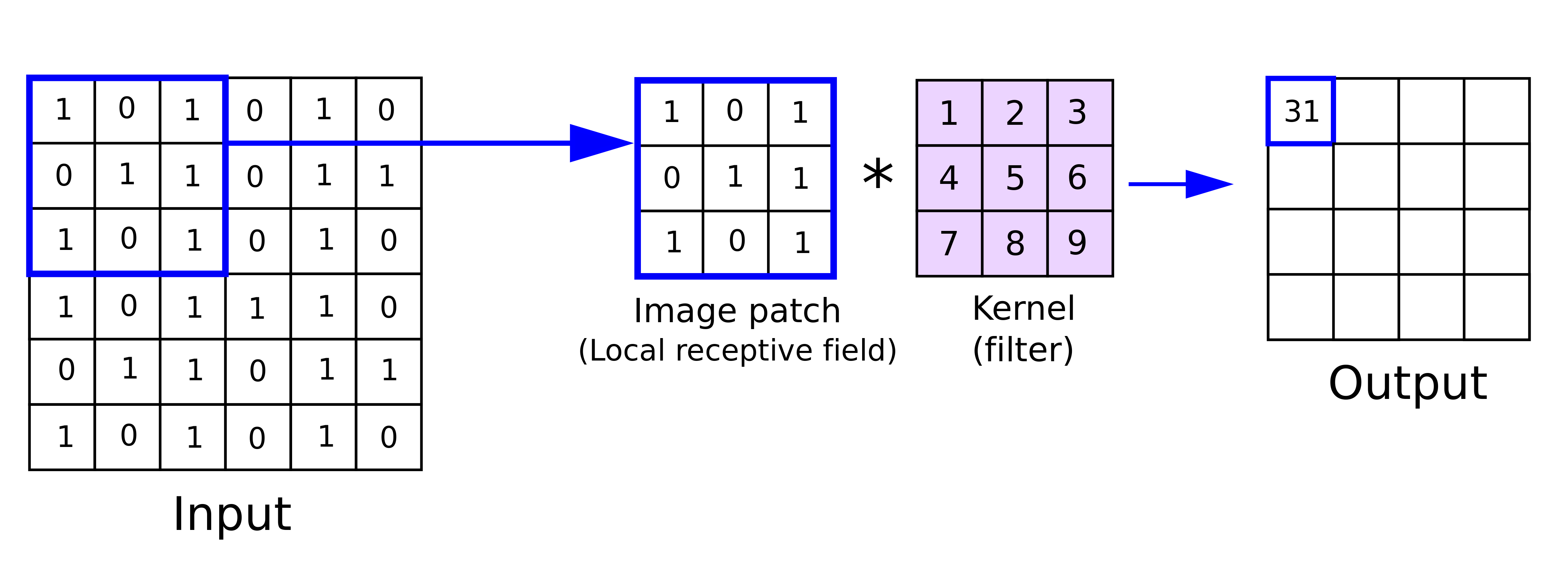

Edge detection

Edge detection is an example of the usefulness of convolution in identifying the regions in an image where there is a sharp change in colors or intesntiy.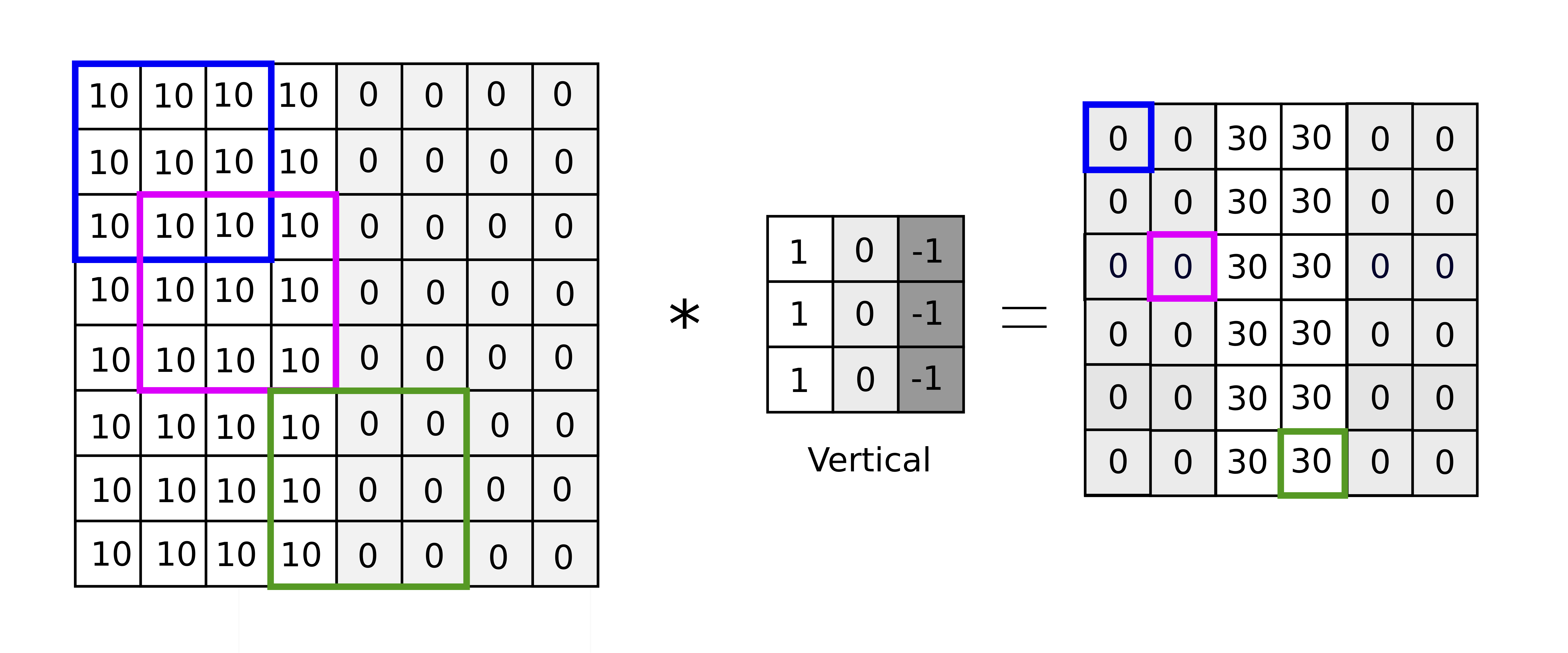

An example of vertical edge detection

For example, in the figure above, applying the convolution operator between the \(3\times 3\) filter (center) and the blue region of the original image (left) gives rise to the element in the new image in blue box (right), whose value can be calculated as the sum of the resulting element-wise product between the 2 matrices: $$ 0 = 10\times 1 + 10\times 0 + 10\times (-1) + 10\times 1 + 10\times 0 + 10\times (-1)\\ + 10\times 1 + 10\times 0 + 10\times (-1)$$
This is an example of a vertical edge detector because it can detect the sharp edge in the middle of the original image, shown by the brighter region in the center of the resulting image.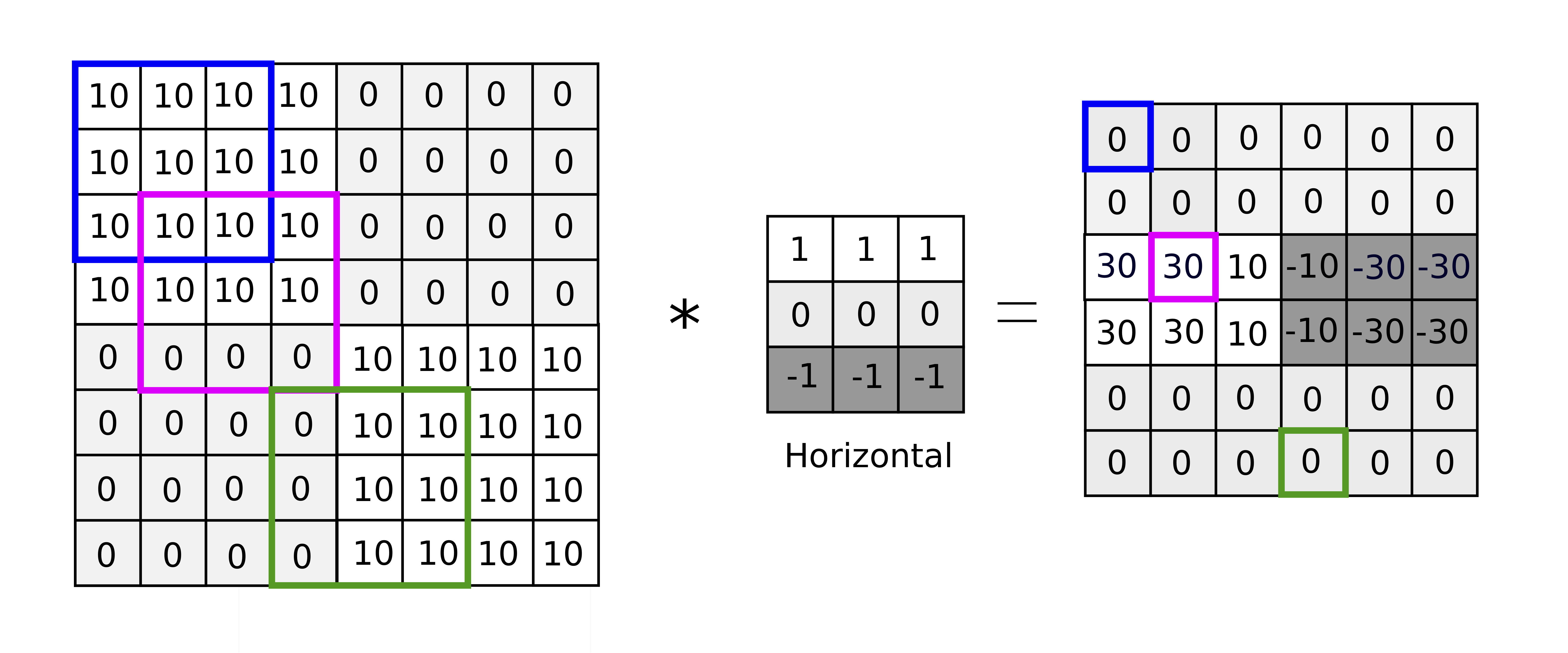

An example of horizontal edge detection

Another example is shown above with a horizontal edge detector with a slightly more complicated image. The non-zero band in the middle reveals the horizontal edge in the center of the original image but also discovers the change from bright to dark (left side) and dark to bright (right side).

Examples of other commonly used filters are shown below. However, instead of hand-picking which filter to use for each task, the parameters associated with the filter from its size to the values of its matrix elements can be trained by a neural network.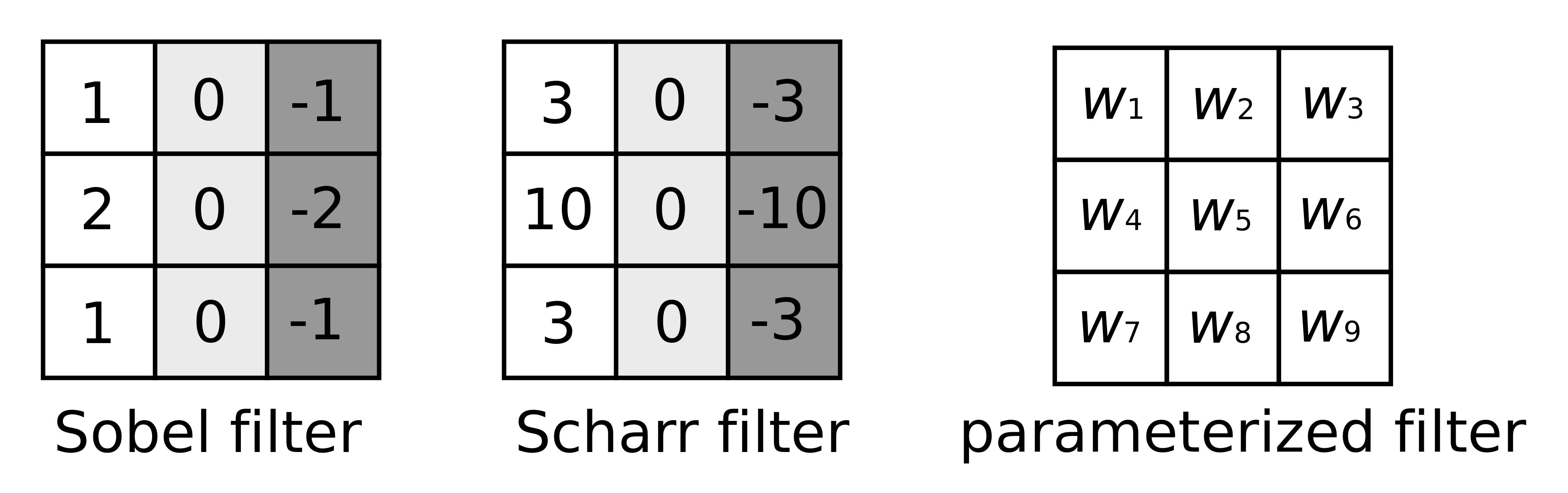

Padding

If the original image is of size \(n\times n\) and the filter is of size \(f\times f\), the size of the resulting image is \( (n–f+1)\times (n–f+1)\). As a result, the input image size is going to shrink after each convolutional layer. In addition, because the edge of the original image is not used in the convolution operation as often as the central pixels, some valuable information is potentially lost in the process.

The solution to these problems is through padding the border of the original image with \(p\) extra layer(s) of zeros in every direction. The dimensions of the input and output images become \((n+2p)\times (n+2p)\) and \((n+2p–f+1)\times(n+2p–f+1)\) respectively. When \(p=0\), that is, no padding, this is called "valid" convolution. When \(p = (f–1)/2\) so that the sizes of the input and output images are the same, this is called "same" convolution.

An example of same convolution with padding \(p=1\)

Convolutional layer

• the convolution operator can be applied to the original image with a stride \(s\) other than 1, resulting in fewer operations and output image of smaller size. $$\left(\frac{n+2p–f}{s}+1\right)\times \left(\frac{n+2p–f}{s}+1\right)$$
• the numbers of channels must be the same for the input image and the filter. See example below for an image with 3 channels (RGB) of dimensions \(6\times 6\times 3\). The filter has dimensions \(3\times 3\times 3\), where the last \(3\) is the number of channels. The resulting image has dimension \(4\times 4\), assuming \(s=1\) and \(p=0\).

• multiple filters can be applied to each image. Given an input image of dimensions \(n\times n\times n_C\) and \(n_C'\) filters of dimensions \(f\times f\times n_C\) with stride \(s\) and padding \(p\), the dimensions of the resulting output is $$\left(\frac{n+2p–f}{s}+1\right)\times \left(\frac{n+2p–f}{s}+1\right)\times n_C'$$
• the number of parameters to be learned in each convolutional layer is \((f\times f\times n_C'+1)\times n_C\), which is independent of the size of the input image. This helps solve the two problems mentioned at the very beginning of this post. Note that \(f, n_C, n_C', p, s\) are all hyperparameters and are not trained in the network, that is, must be tuned outside of the network.

Notation

• For layer \(l\), the filter size, padding, stride are denoted as \(f^{[l]}, p^{[l]}, s^{[l]}\) respectively.
• The dimensions of the input image: \(n_H^{[l–1]}\times n_W^{[l–1]}\times n_C^{[l–1]}\)
• Dimensions of the output image: \(n_H^{[l]}\times n_W^{[l]}\times n_C^{[l]}\)
where $$n_H^{[l]} = \frac{n_H^{[l-1]}+2p^{[l]}-f^{[l]}}{s^{[l]}}+1$$ $$n_W^{[l]} = \frac{n_W^{[l-1]}+2p^{[l]}-f^{[l]}}{s^{[l]}}+1$$ and \(n_C^{[l]}\) is the number of filters used in layer \(l\).
• Size of each filter: \(f^{[l]}\times f^{[l]}\times n_C^{[l–1]}\) (because the number of channels of the filter must match that of the input image)
• Each weight tensor has the same size as a the filter. Since there are \(n_C\) filters, dimensions of the weight tensor \(w^{[l]}\) in layer \(l\) is \(f^{[l]}\times f^{[l]}\times n_C^{[l–1]}\times n_C^{[l]}\), and the bias vector has dimensions \(1\times 1\times 1\times n_C\).
• The activation function \(a^{[l]}\) applies nonlinearity on all the output images, and as a result has dimensions \(m\times n_H^{[l]}\times n_W^{[l]}\times n_C^{[l]}\) where \(m\) is the number of images, that is, the number of training examples.

Pooling layer

The motivation behind pooling layers is to reduce the size of the representation, keeping only the more important features. Pooling layers have been found to work very well, but the underlying reasons for that are not fully understood. The most common type of pooling layers used is Max Pooling; the less common Average Pooling is sometimes seen in very deep neural networks.

Pooling is applied very similarly to the convolution operator by sliding a small matrix of size \(f\times f\) across the input image with stride \(s\). There is almost always no padding, \(p=0\). The Max Pooling operation involves taking the max value, while the Average Pooling, the average. An example is shown for \(f=2\) and \(s=2\) applied on a \(4\times 4\) matrix \((n=4)\). Unlike convolution, pooling is applied to each channel individually, as a result, the number of channels is preserved. The dimensions of the output given input dimensions \(n_H\times n_W\times n_C\) are $$\left(\frac{n_H-f}{s}+1\right)\times \left(\frac{n_W-f}{s}+1\right)\times n_C$$ Since there is no parameter to be learned in a pooling layer, it is often not counted in the number of total layers in a ConvNet.

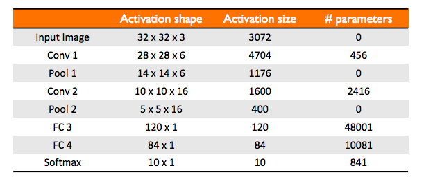
Example of a ConvNet

This simple network that is very similar to LeNet-5 is an example given by Andrew Ng in Course 4 of the Deep Learning Specialization on Coursera. A ConvNet usually consists of a few convolutional layers (each is often followed by a max pooling layer), and a few fully connected layers.


Generally, we can see that \(n_H, n_W\downarrow\) while \(n_C\uparrow\). The size of the activations should gradually decrease. Most of the parameters to be learned in a ConvNet are in the last few fully connected layers as seen in the table below.

The original LeNet-5 was on grey scale images, so the dimensions of the original input image is \(32\times 32\times 1\). In addition, \(tanh\) and \(sigmoid\) activation functions were preferred to ReLU at the time the paper was published.

Why ConvNet?

2 main advantages of using a ConvNet in computer vision applications are

• parameter sharing: a feature detector such as vertical edge detector that is useful in one part of the image is probably be useful in another part of the image. This is often true for both low level features and high level features.
• sparsity of connection: the output unit depends only on a small number of input units. As a result, a ConvNet is more robust and less prone to overfitting.